기존 모델의 한계점
1. 잠재적인 관계를 파악하기 어려운 표 형식 데이터 기반
- 대부분의 변수가 서로 독립적으로 표시되는 표 형식 데이터로는 복잡한 관계를 발견하기 어려움
- 표 형식 데이터는 멀티 오믹스 데이터의 잠재적 관계를 충분히 표현하지 못함
2. 개별 오믹스 데이터 분석을 통한 결과 도출
- 유전체, 전사체, 단백질체, 대사체 등을 개별적으로 분석하여 통합적 이해가 부족
- 생물학적 시스템의 복잡한 상호작용을 포착하기 어려움
3. 복잡한 자연 과정을 설명하는 해석 가능성이 부족한 '블랙박스' 모델
- 기존 딥러닝 모델은 결과는 제공하지만 그 과정에 대한 설명이 부족
- 생물학적 메커니즘에 대한 통찰력 제공이 제한적
4. 데이터 수집 및 모델 선별 비용
- 실제 데이터 수집에 많은 비용과 시간 소요
- 다양한 시나리오에 대한 테스트 어려움
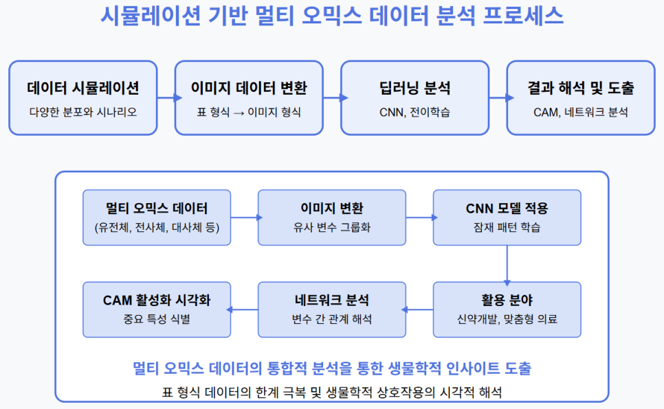
시뮬레이션을 활용한 멀티 오믹스 데이터 분석 프로그램
1. 테이블 형식 오믹스 데이터를 이미지와 같은 표현으로 변환
- CNN(Convolutional Neural Network) 등 딥러닝 모델을 활용하여 잠재적 관계 후보 판별
- 이미지 분석 기법을 적용하여 오믹스 데이터 간의 관계를 보다 잘 파악
2. 전이 학습 활용으로 예측력 향상
- 계산 시간 절약과 분석 정확도 향상 기대
- 소규모 데이터에서도 성능 향상 가능
3. CNN을 활용한 멀티 오믹스 데이터의 예측 모델링
- 기존 기계 학습 기술의 한계 극복과 혁신적 성과 달성 기대
- 풍부한 구조화된 정보 수용 및 이질적인 데이터의 통합적 분석 가능
4. 데이터 시뮬레이션을 통한 데이터 수집 및 모델 선별 비용 절감
- 다양한 분포와 상황을 가정한 데이터를 통한 모델의 일반화 성능 향상
- 특정 시나리오에 대한 모델 성능 사전 테스트로 모델 개발 과정 효율화

데이터 시뮬레이션
- 다양한 분포와 상황을 가정한 데이터를 통한 모델의 일반화 성능 향상
- 여러 가지 생물학적 조건과 환경을 고려한 데이터 생성
- 다양한 시나리오에서의 모델 성능 검증 가능
- 실제 데이터 수집의 한계를 극복하여 충분한 양의 데이터 확보
- 희귀 질환 또는 특수 조건에 대한 데이터 부족 문제 해결
- 데이터 수집 과정의 시간과 비용 절감
- 특정 시나리오에 대한 모델 성능 사전 테스트로 모델 개발 과정 효율화
- 실험 전 가설 검증이 가능하여 연구 방향 설정에 도움
- 모델 개발 전 적합한 데이터 구조와 전처리 방법 확인
이미지 데이터로의 표현
- 표 형식 데이터의 한계 극복
- 대부분 변수가 서로 독립적으로 표시되는 "표 형식" 데이터를 이미지 데이터로 변환
- 이미지 분석 기법을 적용하여 오믹스 데이터 간의 잠재적인 관계를 보다 잘 파악
- 유사 변수의 시각적 그룹화
- 이미지 데이터로 변환하여 유사한 특성을 공유하는 요소를 근접한 이웃 특성으로 배열
- 근접하지 않은 요소는 기존 상태를 유지하면서, CNN이 다각적이고 효율적으로 적용될 수 있는 환경 생성
- 유사한 변수를 가까이 모아 하나의 그룹으로 처리하여 오믹스 데이터의 복잡한 구조와 패턴 반영
- 멀티 오믹스 데이터 통합 표현
- 시뮬레이션으로 얻은 오믹스 데이터들의 정보를 통합하여 표현한 이미지 생성
- 딥러닝을 통해 다양한 오믹스 데이터들 간의 상호 작용을 포착
- 생물 구조적 이해를 촉진하고 분석을 위한 보다 풍부한 내용 제공

이미지 데이터 분석을 위한 딥러닝
- 딥러닝을 이용한 멀티 오믹스 데이터의 관계 추론
- 수많은 상호 작용을 식별하고 비선형 효과를 모델링
- 과적합 위험을 완화할 수 있는 효과적인 정규화 기능 제공
- 오믹스 데이터의 다양한 유형의 구조화된 정보 수용
- 이질적인 데이터를 통합적으로 분석
- 수많은 상호 작용을 식별하고 비선형 효과를 모델링
- 전이 학습
- 딥러닝 모델 구축에 필요한 자원 절약
- 대규모 데이터 세트의 지식을 재사용하여 소규모 데이터에서도 성능 향상 가능
- 사전 훈련된 모델을 새로운 작업에 맞게 특성화하면서 데이터 수집 필요성을 줄이면서도 성능 향상
- 관심영역을 보여주는 CAM(Class Activation Map)
- CAM을 통해 각 클래스(예: 질병 유무, 치료 반응 등)에 대해 모델이 예측할 때 큰 영향을 미치는 이미지의 특정 영역 강조 표시
- 중요한 생물학적 층위나 변수들을 식별하여 모델의 예측 과정을 해석할 수 있게 도움
- 모델의 성능을 개선하거나 모델의 신뢰성을 높이는 데 기여
- 모든 클래스에서 공통적으로 활성화되는 영역을 통해 복잡한 생물학적 네트워크와 상호작용을 통합적으로 이해

네트워크 분석을 통한 인사이트 도출
- 관심 영역의 변수들 간 상관관계, 네트워크 구조 분석
- 생물학적 시스템 내 변수 간 상호작용 이해
- 질병 발생, 치료 반응 등의 복잡한 생물학적 과정을 보다 구체적으로 설명 가능
- 발병 가능성과 관련된 변수 식별
- 양적 관계를 가지는 변수와 음적 관계를 가지는 변수 구분
- 질병 발생 메커니즘에 대한 이해 증진
- 딥러닝을 활용한 모델의 생물학적 해석력 향상
- 블랙박스 모델의 한계 극복
- 예측 결과뿐만 아니라 예측에 기여하는 생물학적 요소 식별
생물학적 시스템 이해 증진
- 다양한 오믹스 데이터의 통합적 분석
- 유전체, 전사체, 단백질체, 대사체 등 다양한 오믹스 데이터를 통합적으로 분석
- 생물학적 시스템의 복잡한 상호작용 이해 증진
- 가설 테스트 및 검증
- 시뮬레이션을 통해 실험적으로 검증하기 어려운 가설에 대한 테스트 및 검증 가능
- Motif Dr 및 WPLite과 같은 신약개발 플랫폼 사용 전, 특정 유전자나 단백질의 구조와 기능 이해 지원
생물학적 시스템 최적화
- 맞춤형 시스템 조절
- 시뮬레이션을 통해 생물학적 시스템의 특정 매개변수를 조절하여 사용자에게 맞춤형 경험 제공
- 다양한 시나리오에 대한 가정과 실험 수행
- 응용 분야
- 유전자 조작, 대사 경로 설계, 약물 개발 등에 활용 가능
- 개인화된 치료법 및 건강 관리 방안 개발 지원
개인 맞춤형 의료 및 건강 관리
- 개인 오믹스 데이터 활용
- 개인의 오믹스 데이터를 분석하고 시뮬레이션하여 질병 예방, 치료, 관리 등에 활용
- 개인의 유전적 특성과 생활 습관을 고려한 맞춤형 의료 서비스 제공
- 신약 후보 물질 발굴
- AD3 및 AI Drug 플랫폼 등에서 신약 후보 물질을 더욱 정밀하게 발굴하도록 지원
- 개인별 약물 반응 예측 및 최적화
실습용 코드
멀티오믹스 데이터 이미지 변환 및 CNN 분석 튜토리얼
"""
멀티 오믹스 데이터 이미지 변환 및 CNN 분석 튜토리얼
=====================================================
이 코드는 다음 단계를 포함합니다:
1. 멀티 오믹스 데이터 시뮬레이션
2. 표 형식 데이터를 이미지로 변환 (DeepInsight 접근법)
3. CNN 모델 구축 및 학습
4. Class Activation Map(CAM)을 통한 해석
5. 네트워크 분석을 통한 중요 특성 식별
"""
import numpy as np
import pandas as pd
import matplotlib.pyplot as plt
import seaborn as sns
from sklearn.preprocessing import StandardScaler
from sklearn.manifold import TSNE
from sklearn.model_selection import train_test_split
from sklearn.metrics import classification_report, confusion_matrix, roc_curve, auc
import networkx as nx
import tensorflow as tf
from tensorflow.keras.models import Model, Sequential
from tensorflow.keras.layers import Dense, Dropout, Flatten, Conv2D, MaxPooling2D, Input, BatchNormalization
from tensorflow.keras.utils import to_categorical
from tensorflow.keras.callbacks import EarlyStopping, ModelCheckpoint
# 경고 메시지 숨기기
import warnings
warnings.filterwarnings('ignore')
# 결과 재현성을 위한 시드 설정
np.random.seed(42)
tf.random.set_seed(42)
#----------------------------------------------------
# 1. 멀티 오믹스 데이터 시뮬레이션
#----------------------------------------------------
def simulate_multiomics_data(n_samples=1000, n_genomics=200, n_transcriptomics=300,
n_proteomics=150, n_metabolomics=100, n_classes=2):
"""
멀티 오믹스 데이터(유전체, 전사체, 단백질체, 대사체)를 시뮬레이션합니다.
Parameters:
-----------
n_samples : int
샘플 수
n_genomics, n_transcriptomics, n_proteomics, n_metabolomics : int
각 오믹스 계층의 특성 수
n_classes : int
질병 상태 등의 클래스 수
Returns:
--------
X_multiomics : pandas.DataFrame
시뮬레이션된 멀티 오믹스 데이터
y : numpy.ndarray
클래스 레이블
"""
# 각 오믹스 계층의 특성 수 설정
n_features = n_genomics + n_transcriptomics + n_proteomics + n_metabolomics
# 상관 관계가 있는 특성 생성 - 생물학적 네트워크를 모방
# 공분산 행렬 생성
correlation_matrix = np.eye(n_features)
# 유전체 내부 상관관계
for i in range(n_genomics):
for j in range(i+1, n_genomics):
if np.random.random() < 0.1: # 10% 확률로 상관관계 생성
correlation_val = np.random.uniform(0.3, 0.7)
correlation_matrix[i, j] = correlation_val
correlation_matrix[j, i] = correlation_val
# 전사체와 유전체 간 상관관계
for i in range(n_genomics):
for j in range(n_genomics, n_genomics + n_transcriptomics):
if np.random.random() < 0.15: # 15% 확률로 상관관계 생성
correlation_val = np.random.uniform(0.4, 0.8)
correlation_matrix[i, j] = correlation_val
correlation_matrix[j, i] = correlation_val
# 단백질체와 전사체 간 상관관계
for i in range(n_genomics, n_genomics + n_transcriptomics):
for j in range(n_genomics + n_transcriptomics, n_genomics + n_transcriptomics + n_proteomics):
if np.random.random() < 0.2: # 20% 확률로 상관관계 생성
correlation_val = np.random.uniform(0.5, 0.9)
correlation_matrix[i, j] = correlation_val
correlation_matrix[j, i] = correlation_val
# 대사체와 단백질체 간 상관관계
for i in range(n_genomics + n_transcriptomics, n_genomics + n_transcriptomics + n_proteomics):
for j in range(n_genomics + n_transcriptomics + n_proteomics, n_features):
if np.random.random() < 0.25: # 25% 확률로 상관관계 생성
correlation_val = np.random.uniform(0.6, 0.95)
correlation_matrix[i, j] = correlation_val
correlation_matrix[j, i] = correlation_val
# 공분산 행렬이 positive definite가 되도록 조정
min_eigval = np.min(np.linalg.eigvals(correlation_matrix))
if min_eigval < 0:
correlation_matrix += (-min_eigval + 0.01) * np.eye(n_features)
# 다변량 정규 분포에서 특성 생성
X = np.random.multivariate_normal(mean=np.zeros(n_features), cov=correlation_matrix, size=n_samples)
# 클래스 생성에 영향을 미치는 특성 선택 (각 오믹스에서 일부 선택)
n_influential_features = 50
influential_indices = np.random.choice(n_features, size=n_influential_features, replace=False)
# 클래스 레이블 생성
prob = 1 / (1 + np.exp(-np.sum(X[:, influential_indices] * np.random.uniform(-2, 2, n_influential_features), axis=1)))
y = (prob > 0.5).astype(int)
if n_classes > 2:
# 다중 클래스 시나리오
y = np.floor(prob * n_classes).astype(int)
y = np.clip(y, 0, n_classes - 1) # 경계 확인
# 잡음 추가
X = X + np.random.normal(0, 0.1, X.shape)
# 데이터프레임 생성
feature_names = []
feature_names += [f'gene_{i}' for i in range(n_genomics)]
feature_names += [f'transcript_{i}' for i in range(n_transcriptomics)]
feature_names += [f'protein_{i}' for i in range(n_proteomics)]
feature_names += [f'metabolite_{i}' for i in range(n_metabolomics)]
X_multiomics = pd.DataFrame(X, columns=feature_names)
# 영향력 있는 특성 정보 저장 (나중에 해석에 사용)
influential_features = [feature_names[idx] for idx in influential_indices]
return X_multiomics, y, influential_features
[출처] 인공지능신약개발활용 실습|작성자 말러83
# DeepInsight 접근법
#----------------------------------------------------
# 2. 표 형식 데이터를 이미지로 변환 (DeepInsight 접근법)
#----------------------------------------------------
class DeepInsightTransformer:
"""
DeepInsight 방법을 사용하여 표 형식 데이터를 이미지로 변환합니다.
이 방법은 t-SNE나 다른 차원 축소 기법을 사용하여 특성을 2D 공간에 배치합니다.
Reference:
Sharma, A., Vans, E., Shigemizu, D. et al.
DeepInsight: A methodology to transform a non-image data to an image for convolution neural network architecture.
Sci Rep 9, 11399 (2019).
"""
def __init__(self, image_size=100, perplexity=30, random_state=42):
"""
Parameters:
-----------
image_size : int
생성할 이미지의 크기 (너비와 높이)
perplexity : int
t-SNE 알고리즘의 perplexity 파라미터
random_state : int
재현성을 위한 랜덤 시드
"""
self.image_size = image_size
self.perplexity = perplexity
self.random_state = random_state
self.pixel_coords = None
self.scaler = StandardScaler()
self.feature_names = None
def fit(self, X):
"""
X의 특성을 t-SNE를 사용하여 2D 이미지 좌표에 매핑합니다.
Parameters:
-----------
X : pandas.DataFrame or numpy.ndarray
변환할 데이터
Returns:
--------
self
"""
if isinstance(X, pd.DataFrame):
self.feature_names = X.columns
X_numeric = X.values
else:
X_numeric = X
self.feature_names = [f"feature_{i}" for i in range(X.shape[1])]
# 데이터 스케일링
X_scaled = self.scaler.fit_transform(X_numeric)
# t-SNE를 사용하여 특성을 2D에 매핑
tsne = TSNE(n_components=2, perplexity=self.perplexity, random_state=self.random_state)
feature_coords = tsne.fit_transform(X_scaled.T) # 특성에 대해 t-SNE 적용
# 이미지 좌표로 스케일링
min_coords = np.min(feature_coords, axis=0)
max_coords = np.max(feature_coords, axis=0)
feature_coords = (feature_coords - min_coords) / (max_coords - min_coords)
# 이미지 픽셀 좌표 계산
pixel_coords = np.floor(feature_coords * (self.image_size - 1)).astype(int)
# 중복 좌표 처리
unique_coords, unique_indices = np.unique(pixel_coords, return_index=True, axis=0)
if len(unique_coords) < len(pixel_coords):
print(f"경고: {len(pixel_coords) - len(unique_coords)}개의 중복 좌표가 발생했습니다. 근접한 좌표로 조정합니다.")
# 중복된 좌표에 작은 오프셋 추가
duplicated_mask = np.ones(len(pixel_coords), dtype=bool)
duplicated_mask[unique_indices] = False
for idx in np.where(duplicated_mask)[0]:
while True:
offset = np.random.randint(-1, 2, size=2)
new_coord = pixel_coords[idx] + offset
if (new_coord[0] >= 0 and new_coord[0] < self.image_size and
new_coord[1] >= 0 and new_coord[1] < self.image_size and
not np.any(np.all(new_coord == pixel_coords, axis=1))):
pixel_coords[idx] = new_coord
break
self.pixel_coords = pixel_coords
return self
def transform(self, X):
"""
특성 값을 사용하여 이미지로 변환합니다.
Parameters:
-----------
X : pandas.DataFrame or numpy.ndarray
변환할 데이터
Returns:
--------
images : numpy.ndarray
변환된 이미지 (samples, height, width, 1)
"""
if self.pixel_coords is None:
raise ValueError("transform 전에 fit을 호출해야 합니다.")
if isinstance(X, pd.DataFrame):
X_numeric = X.values
else:
X_numeric = X
# 데이터 스케일링
X_scaled = self.scaler.transform(X_numeric)
# 이미지 생성
n_samples = X_scaled.shape[0]
images = np.zeros((n_samples, self.image_size, self.image_size, 1))
for sample_idx in range(n_samples):
for feature_idx, (x, y) in enumerate(self.pixel_coords):
images[sample_idx, y, x, 0] = X_scaled[sample_idx, feature_idx]
return images
def fit_transform(self, X):
"""
fit과 transform을 연속으로 수행합니다.
"""
return self.fit(X).transform(X)
def get_feature_locations(self):
"""
각 특성의 이미지 상의 위치를 반환합니다.
Returns:
--------
feature_locations : dict
특성 이름을 키로, (x, y) 좌표를 값으로 갖는 딕셔너리
"""
if self.pixel_coords is None:
raise ValueError("fit을 먼저 호출해야 합니다.")
feature_locations = {}
for i, feat_name in enumerate(self.feature_names):
feature_locations[feat_name] = tuple(self.pixel_coords[i])
return feature_locations
def visualize_feature_map(self, figsize=(10, 10)):
"""
특성의 2D 맵을 시각화합니다.
Parameters:
#----------------------------------------------------
# 2. 표 형식 데이터를 이미지로 변환 (DeepInsight 접근법)
#----------------------------------------------------
class DeepInsightTransformer:
"""
DeepInsight 방법을 사용하여 표 형식 데이터를 이미지로 변환합니다.
이 방법은 t-SNE나 다른 차원 축소 기법을 사용하여 특성을 2D 공간에 배치합니다.
Reference:
Sharma, A., Vans, E., Shigemizu, D. et al.
DeepInsight: A methodology to transform a non-image data to an image for convolution neural network architecture.
Sci Rep 9, 11399 (2019).
"""
def __init__(self, image_size=100, perplexity=30, random_state=42):
"""
Parameters:
-----------
image_size : int
생성할 이미지의 크기 (너비와 높이)
perplexity : int
t-SNE 알고리즘의 perplexity 파라미터
random_state : int
재현성을 위한 랜덤 시드
"""
self.image_size = image_size
self.perplexity = perplexity
self.random_state = random_state
self.pixel_coords = None
self.scaler = StandardScaler()
self.feature_names = None
def fit(self, X):
"""
X의 특성을 t-SNE를 사용하여 2D 이미지 좌표에 매핑합니다.
Parameters:
-----------
X : pandas.DataFrame or numpy.ndarray
변환할 데이터
Returns:
--------
self
"""
if isinstance(X, pd.DataFrame):
self.feature_names = X.columns
X_numeric = X.values
else:
X_numeric = X
self.feature_names = [f"feature_{i}" for i in range(X.shape[1])]
# 데이터 스케일링
X_scaled = self.scaler.fit_transform(X_numeric)
# t-SNE를 사용하여 특성을 2D에 매핑
tsne = TSNE(n_components=2, perplexity=self.perplexity, random_state=self.random_state)
feature_coords = tsne.fit_transform(X_scaled.T) # 특성에 대해 t-SNE 적용
# 이미지 좌표로 스케일링
min_coords = np.min(feature_coords, axis=0)
max_coords = np.max(feature_coords, axis=0)
feature_coords = (feature_coords - min_coords) / (max_coords - min_coords)
# 이미지 픽셀 좌표 계산
pixel_coords = np.floor(feature_coords * (self.image_size - 1)).astype(int)
# 중복 좌표 처리
unique_coords, unique_indices = np.unique(pixel_coords, return_index=True, axis=0)
if len(unique_coords) < len(pixel_coords):
print(f"경고: {len(pixel_coords) - len(unique_coords)}개의 중복 좌표가 발생했습니다. 근접한 좌표로 조정합니다.")
# 중복된 좌표에 작은 오프셋 추가
duplicated_mask = np.ones(len(pixel_coords), dtype=bool)
duplicated_mask[unique_indices] = False
for idx in np.where(duplicated_mask)[0]:
while True:
offset = np.random.randint(-1, 2, size=2)
new_coord = pixel_coords[idx] + offset
if (new_coord[0] >= 0 and new_coord[0] < self.image_size and
new_coord[1] >= 0 and new_coord[1] < self.image_size and
not np.any(np.all(new_coord == pixel_coords, axis=1))):
pixel_coords[idx] = new_coord
break
self.pixel_coords = pixel_coords
return self
def transform(self, X):
"""
특성 값을 사용하여 이미지로 변환합니다.
Parameters:
-----------
X : pandas.DataFrame or numpy.ndarray
변환할 데이터
Returns:
--------
images : numpy.ndarray
변환된 이미지 (samples, height, width, 1)
"""
if self.pixel_coords is None:
raise ValueError("transform 전에 fit을 호출해야 합니다.")
if isinstance(X, pd.DataFrame):
X_numeric = X.values
else:
X_numeric = X
# 데이터 스케일링
X_scaled = self.scaler.transform(X_numeric)
# 이미지 생성
n_samples = X_scaled.shape[0]
images = np.zeros((n_samples, self.image_size, self.image_size, 1))
for sample_idx in range(n_samples):
for feature_idx, (x, y) in enumerate(self.pixel_coords):
images[sample_idx, y, x, 0] = X_scaled[sample_idx, feature_idx]
return images
def fit_transform(self, X):
"""
fit과 transform을 연속으로 수행합니다.
"""
return self.fit(X).transform(X)
def get_feature_locations(self):
"""
각 특성의 이미지 상의 위치를 반환합니다.
Returns:
--------
feature_locations : dict
특성 이름을 키로, (x, y) 좌표를 값으로 갖는 딕셔너리
"""
if self.pixel_coords is None:
raise ValueError("fit을 먼저 호출해야 합니다.")
feature_locations = {}
for i, feat_name in enumerate(self.feature_names):
feature_locations[feat_name] = tuple(self.pixel_coords[i])
return feature_locations
def visualize_feature_map(self, figsize=(10, 10)):
"""
특성의 2D 맵을 시각화합니다.
Parameters:
# CNN 모델 구축
#----------------------------------------------------
# 3. CNN 모델 구축 및 학습
#----------------------------------------------------
def build_cnn_model(input_shape=(100, 100, 1), num_classes=2):
"""
멀티 오믹스 이미지 분류를 위한 CNN 모델을 구축합니다.
Parameters:
-----------
input_shape : tuple
입력 이미지 형태 (height, width, channels)
num_classes : int
분류할 클래스 수
Returns:
--------
model : tensorflow.keras.Model
구축된 CNN 모델
"""
inputs = Input(shape=input_shape)
# 첫 번째 컨볼루션 블록
x = Conv2D(32, (3, 3), activation='relu', padding='same')(inputs)
x = BatchNormalization()(x)
x = MaxPooling2D((2, 2))(x)
# 두 번째 컨볼루션 블록
x = Conv2D(64, (3, 3), activation='relu', padding='same')(x)
x = BatchNormalization()(x)
x = MaxPooling2D((2, 2))(x)
# 세 번째 컨볼루션 블록
x = Conv2D(128, (3, 3), activation='relu', padding='same')(x)
x = BatchNormalization()(x)
x = MaxPooling2D((2, 2))(x)
# 추가 레이어 - Grad-CAM에서 사용할 레이어
last_conv_layer = Conv2D(64, (3, 3), activation='relu', padding='same', name='last_conv')(x)
x = MaxPooling2D((2, 2))(last_conv_layer)
# 완전연결 레이어
x = Flatten()(x)
x = Dense(128, activation='relu')(x)
x = Dropout(0.5)(x)
if num_classes == 2:
outputs = Dense(1, activation='sigmoid')(x)
loss = 'binary_crossentropy'
else:
outputs = Dense(num_classes, activation='softmax')(x)
loss = 'categorical_crossentropy'
model = Model(inputs=inputs, outputs=outputs)
# 모델 컴파일
model.compile(
optimizer='adam',
loss=loss,
metrics=['accuracy']
)
return model
#----------------------------------------------------
# 3. CNN 모델 구축 및 학습
#----------------------------------------------------
def build_cnn_model(input_shape=(100, 100, 1), num_classes=2):
"""
멀티 오믹스 이미지 분류를 위한 CNN 모델을 구축합니다.
Parameters:
-----------
input_shape : tuple
입력 이미지 형태 (height, width, channels)
num_classes : int
분류할 클래스 수
Returns:
--------
model : tensorflow.keras.Model
구축된 CNN 모델
"""
inputs = Input(shape=input_shape)
# 첫 번째 컨볼루션 블록
x = Conv2D(32, (3, 3), activation='relu', padding='same')(inputs)
x = BatchNormalization()(x)
x = MaxPooling2D((2, 2))(x)
# 두 번째 컨볼루션 블록
x = Conv2D(64, (3, 3), activation='relu', padding='same')(x)
x = BatchNormalization()(x)
x = MaxPooling2D((2, 2))(x)
# 세 번째 컨볼루션 블록
x = Conv2D(128, (3, 3), activation='relu', padding='same')(x)
x = BatchNormalization()(x)
x = MaxPooling2D((2, 2))(x)
# 추가 레이어 - Grad-CAM에서 사용할 레이어
last_conv_layer = Conv2D(64, (3, 3), activation='relu', padding='same', name='last_conv')(x)
x = MaxPooling2D((2, 2))(last_conv_layer)
# 완전연결 레이어
x = Flatten()(x)
x = Dense(128, activation='relu')(x)
x = Dropout(0.5)(x)
if num_classes == 2:
outputs = Dense(1, activation='sigmoid')(x)
loss = 'binary_crossentropy'
else:
outputs = Dense(num_classes, activation='softmax')(x)
loss = 'categorical_crossentropy'
model = Model(inputs=inputs, outputs=outputs)
# 모델 컴파일
model.compile(
optimizer='adam',
loss=loss,
metrics=['accuracy']
)
return model
# CAM 해석
#----------------------------------------------------
# 4. Class Activation Map(CAM)을 통한 해석
#----------------------------------------------------
def generate_grad_cam(model, image, class_idx=None, layer_name='last_conv'):
"""
Grad-CAM(Gradient-weighted Class Activation Mapping)을 생성합니다.
Parameters:
-----------
model : tensorflow.keras.Model
학습된 CNN 모델
image : numpy.ndarray
시각화할 이미지 (1, height, width, channels)
class_idx : int, optional
시각화할 클래스 인덱스 (기본값은 가장 높은 예측 확률을 가진 클래스)
layer_name : str
Grad-CAM을 생성할 레이어 이름
Returns:
--------
cam : numpy.ndarray
클래스 활성화 맵
"""
# 모델에서 지정한 레이어 가져오기
grad_model = Model(
inputs=[model.inputs],
outputs=[model.get_layer(layer_name).output, model.output]
)
# 이미지를 모델에 넣고 그래디언트 계산
with tf.GradientTape() as tape:
conv_outputs, predictions = grad_model(image)
if class_idx is None:
if predictions.shape[-1] > 1:
class_idx = tf.argmax(predictions[0])
else:
class_idx = 0 # 이진 분류의 경우
if predictions.shape[-1] > 1:
loss = predictions[:, class_idx]
else:
loss = predictions[0] # 이진 분류의 경우
# 출력에 대한 그래디언트 계산
grads = tape.gradient(loss, conv_outputs)
# 채널별 평균 그래디언트 계산 (중요도)
pooled_grads = tf.reduce_mean(grads, axis=(0, 1, 2))
# 특성 맵과 가중치를 곱함
conv_outputs = conv_outputs[0]
cam = tf.reduce_sum(tf.multiply(pooled_grads, conv_outputs), axis=-1)
# CAM을 원래 이미지 크기로 조정 및 ReLU 적용
cam = np.maximum(cam, 0) # ReLU 적용
cam = cam / np.max(cam) # 0-1 사이로 정규화
# 원본 이미지 크기로 리사이즈
h, w = image.shape[1:3]
cam = tf.image.resize(tf.expand_dims(tf.expand_dims(cam, 0), -1), (h, w))[0, :, :, 0].numpy()
return cam
def visualize_grad_cam(image, cam, alpha=0.5, cmap='jet', figsize=(12, 4)):
"""
원본 이미지와 Grad-CAM을 시각화합니다.
Parameters:
-----------
image : numpy.ndarray
원본 이미지 (height, width, channels)
cam : numpy.ndarray
클래스 활성화 맵
alpha : float
오버레이 투명도
cmap : str
캠 컬러맵
figsize : tuple
그림 크기
"""
plt.figure(figsize=figsize)
# 원본 이미지
plt.subplot(1, 3, 1)
plt.imshow(image[:, :, 0], cmap='gray')
plt.title('원본 변환 이미지')
plt.axis('off')
# CAM
plt.subplot(1, 3, 2)
plt.imshow(cam, cmap=cmap)
plt.title('Grad-CAM')
plt.axis('off')
plt.colorbar(label='활성화 강도')
# 오버레이
plt.subplot(1, 3, 3)
# 원본 이미지를 RGB로 변환
if image.shape[-1] == 1:
rgb_img = np.repeat(image, 3, axis=2)
else:
rgb_img = image
# CAM을 heatmap으로 변환
import matplotlib.cm as cm
heatmap = cm.get_cmap(cmap)(cam)[:, :, :3] # RGBA에서 RGB로 변환
# 오버레이 생성
overlay = rgb_img * (1 - alpha) + heatmap * alpha
overlay = np.clip(overlay, 0, 1) # 값 클리핑
plt.imshow(overlay)
plt.title('CAM 오버레이')
plt.axis('off')
plt.tight_layout()
plt.show()
# 네트워크 분석
#----------------------------------------------------
# 5. 네트워크 분석을 통한 중요 특성 식별
#----------------------------------------------------
def analyze_feature_importance(transformer, grad_cam_results, top_n=20):
"""
Grad-CAM 결과와 특성 위치를 기반으로 중요 특성을 식별합니다.
Parameters:
-----------
transformer : DeepInsightTransformer
DeepInsight 변환기
grad_cam_results : numpy.ndarray
Grad-CAM 결과 (height, width)
top_n : int
반환할 상위 특성 수
Returns:
--------
top_features : list
중요도 순으로 정렬된 (특성 이름, 중요도) 튜플 리스트
"""
feature_locations = transformer.get_feature_locations()
feature_importance = {}
for feature_name, (x, y) in feature_locations.items():
# 좌표가 Grad-CAM 크기 범위 내에 있는지 확인
if y < grad_cam_results.shape[0] and x < grad_cam_results.shape[1]:
importance = grad_cam_results[y, x]
feature_importance[feature_name] = importance
# 중요도 순으로 정렬
sorted_features = sorted(feature_importance.items(), key=lambda x: x[1], reverse=True)
top_features = sorted_features[:top_n]
return top_features
def create_feature_network(X, top_features, threshold=0.3):
"""
중요 특성 간의 상관관계 네트워크를 생성합니다.
Parameters:
-----------
X : pandas.DataFrame
원본 데이터
top_features : list
중요 특성 리스트 (이름, 중요도)
threshold : float
네트워크에 포함할 상관관계 임계값
Returns:
--------
G : networkx.Graph
특성 네트워크
"""
feature_names = [f[0] for f in top_features]
X_selected = X[feature_names]
# 상관관계 계산
corr_matrix = X_selected.corr().abs()
# 네트워크 생성
G = nx.Graph()
# 노드 추가 (특성 중요도 정보 포함)
for feature, importance in top_features:
G.add_node(feature, importance=importance)
# 엣지 추가
for i, feature1 in enumerate(feature_names):
for j, feature2 in enumerate(feature_names[i+1:], i+1):
correlation = corr_matrix.loc[feature1, feature2]
if correlation > threshold:
G.add_edge(feature1, feature2, weight=correlation)
return G
def visualize_feature_network(G, figsize=(12, 12)):
"""
특성 네트워크를 시각화합니다.
Parameters:
-----------
G : networkx.Graph
특성 네트워크
figsize : tuple
그림 크기
"""
plt.figure(figsize=figsize)
# 노드 위치 계산
pos = nx.spring_layout(G, seed=42)
# 노드 중요도에 따른 크기
node_importance = nx.get_node_attributes(G, 'importance')
node_size = [v * 1000 + 100 for v in node_importance.values()]
# 엣지 가중치
edge_weights = nx.get_edge_attributes(G, 'weight')
edge_width = [w * 2 for w in edge_weights.values()]
# 노드 그룹화 (오믹스 타입별)
genomic_nodes = [n for n in G.nodes() if 'gene_' in n]
transcript_nodes = [n for n in G.nodes() if 'transcript_' in n]
protein_nodes = [n for n in G.nodes() if 'protein_' in n]
metabolite_nodes = [n for n in G.nodes() if 'metabolite_' in n]
# 네트워크 시각화
nx.draw_networkx_nodes(G, pos, nodelist=genomic_nodes, node_size=node_size,
node_color='skyblue', alpha=0.8, label='Genomic')
#----------------------------------------------------
# 5. 네트워크 분석을 통한 중요 특성 식별
#----------------------------------------------------
def analyze_feature_importance(transformer, grad_cam_results, top_n=20):
"""
Grad-CAM 결과와 특성 위치를 기반으로 중요 특성을 식별합니다.
Parameters:
-----------
transformer : DeepInsightTransformer
DeepInsight 변환기
grad_cam_results : numpy.ndarray
Grad-CAM 결과 (height, width)
top_n : int
반환할 상위 특성 수
Returns:
--------
top_features : list
중요도 순으로 정렬된 (특성 이름, 중요도) 튜플 리스트
"""
feature_locations = transformer.get_feature_locations()
feature_importance = {}
for feature_name, (x, y) in feature_locations.items():
# 좌표가 Grad-CAM 크기 범위 내에 있는지 확인
if y < grad_cam_results.shape[0] and x < grad_cam_results.shape[1]:
importance = grad_cam_results[y, x]
feature_importance[feature_name] = importance
# 중요도 순으로 정렬
sorted_features = sorted(feature_importance.items(), key=lambda x: x[1], reverse=True)
top_features = sorted_features[:top_n]
return top_features
def create_feature_network(X, top_features, threshold=0.3):
"""
중요 특성 간의 상관관계 네트워크를 생성합니다.
Parameters:
-----------
X : pandas.DataFrame
원본 데이터
top_features : list
중요 특성 리스트 (이름, 중요도)
threshold : float
네트워크에 포함할 상관관계 임계값
Returns:
--------
G : networkx.Graph
특성 네트워크
"""
feature_names = [f[0] for f in top_features]
X_selected = X[feature_names]
# 상관관계 계산
corr_matrix = X_selected.corr().abs()
# 네트워크 생성
G = nx.Graph()
# 노드 추가 (특성 중요도 정보 포함)
for feature, importance in top_features:
G.add_node(feature, importance=importance)
# 엣지 추가
for i, feature1 in enumerate(feature_names):
for j, feature2 in enumerate(feature_names[i+1:], i+1):
correlation = corr_matrix.loc[feature1, feature2]
if correlation > threshold:
G.add_edge(feature1, feature2, weight=correlation)
return G
def visualize_feature_network(G, figsize=(12, 12)):
"""
특성 네트워크를 시각화합니다.
Parameters:
-----------
G : networkx.Graph
특성 네트워크
figsize : tuple
그림 크기
"""
plt.figure(figsize=figsize)
# 노드 위치 계산
pos = nx.spring_layout(G, seed=42)
# 노드 중요도에 따른 크기
node_importance = nx.get_node_attributes(G, 'importance')
node_size = [v * 1000 + 100 for v in node_importance.values()]
# 엣지 가중치
edge_weights = nx.get_edge_attributes(G, 'weight')
edge_width = [w * 2 for w in edge_weights.values()]
# 노드 그룹화 (오믹스 타입별)
genomic_nodes = [n for n in G.nodes() if 'gene_' in n]
transcript_nodes = [n for n in G.nodes() if 'transcript_' in n]
protein_nodes = [n for n in G.nodes() if 'protein_' in n]
metabolite_nodes = [n for n in G.nodes() if 'metabolite_' in n]
# 네트워크 시각화
nx.draw_networkx_nodes(G, pos, nodelist=genomic_nodes, node_size=node_size,
node_color='skyblue', alpha=0.8, label='Genomic')